The final day of Julia is a lot more challenging than the first 2 — consisting of a larger example of some image processing and a little bit about macros along with some wrap up material and some challenging exercises.
Throughout the whole thing Julia struck me as a very usable language. Intuitive, nicely structured and with just enough syntax to make it very pleasant to use. The quote from Graydon Hoare is very aposite — he calls Julia a Goldilocks language
because the designers have got it just right
Exercises
Easy exercises
Write a macro that runs a block of code backwards
Not quite sure what running code backwards really means here. I just deconstruct an expression, reverse its arguments and map eval over that. I suppose that is what was required.
julia> macro backwards(b)
         quote
           map(eval,reverse($b.args))
           return
         end
       end

julia> @backwards :(begin
           println("one")
           println("two")
       end)
two
one
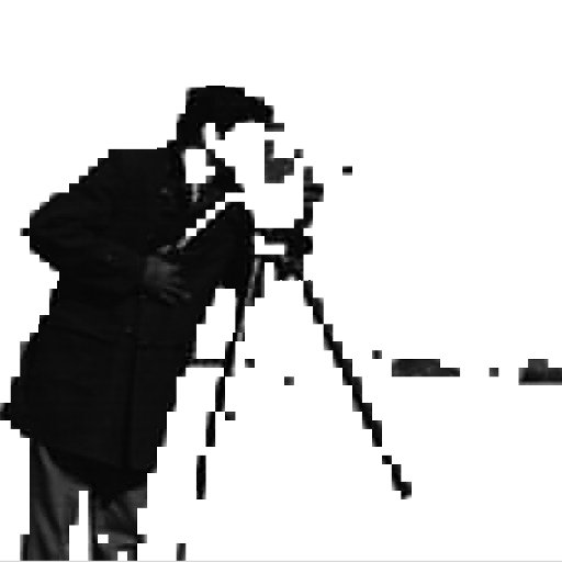
Experiment with modifying frequencies and observing the effect on an image. What happens when you set some high frequencies to large values?
Scaling up the higher numbers makes the image background much less detailed, effectively it ends up being white as you can see from the picture. My implementation is below.
function blockdct6(img)
  pixels = convert(Array{Float32}, img.data)
  y,x = size(pixels)

  outx = ifloor(x/8)
  outy = ifloor(y/8)

  bx = 1:8:outx*8
  by = 1:8:outy*8

  mask = zeros(8,8)
  mask[1:3,1:3] = [1 1 1; 1 1 0; 1 0 0]  ## keep stuff marked 1, drop stuff that is 0

  freqs = Array(Float32, (outy*8,outx*8))

  for i=bx, j=by
    freqs[j:j+7, i:i+7] = dct(pixels[j:j+7, i:i+7])
    freqs[j:j+7, i:i+7] .*= mask
  end

  map(scaleupHighNumber, freqs)
end

function scaleupHighNumber(n)
  if n > 2
    n * 144
  else
    n
  end
end
What happens if you add lots of noise? (Hint: try adding scale * rand(size(freqs))
As you can see, adding noise makes the image look significantly blockier.
Here is how I did that.
function blockdct6(img)
  pixels = convert(Array{Float32}, img.data)
  y,x = size(pixels)

  outx = ifloor(x/8)
  outy = ifloor(y/8)

  bx = 1:8:outx*8
  by = 1:8:outy*8

  mask = zeros(8,8)
  mask[1:3,1:3] = [1 1 1; 1 1 0; 1 0 0]  ## keep stuff marked 1, drop stuff that is 0

  freqs = Array(Float32, (outy*8,outx*8))

  for i=bx, j=by
    freqs[j:j+7, i:i+7] = dct(pixels[j:j+7, i:i+7])
    freqs[j:j+7, i:i+7] .*= mask
  end

  freqs .* rand(size(freqs))
end
Medium exercises
Modify the code to allow masking arbitrarily many coefficient, but always the N most important ones. Instead of calling blockdct6(img), you would call blockdct(img,6)
In implementing this one, I made the assumption that arbitrarily many
would be bounded by our block size, so up a maximum of to 8x8 == 64 cells could be masked by calling make_mask(16) as we are working with 8x8 blocks. The algorithim could remain substantially the same, if you wanted to support different sized blocks.
I make a subsidiary function to deal with the mask making, it takes the width of the block being processed and an n for the number of "significant" coefficients.
function make_mask(width,n)
  row_max = n
  arr=zeros(width,width)
  println(arr)
  for i=1:row_max
     for j=1:row_max
        if(j<n-(i+1))
          arr[i,j]=1
        end
     end
  end
  arr
end

function blockdct(img, n)
  pixels = convert(Array{Float32}, img.data)
  y,x = size(pixels)

  outx = ifloor(x/8)
  outy = ifloor(y/8)

  bx = 1:8:outx*8
  by = 1:8:outy*8

  mask = make_mask(8,n)

  freqs = Array(Float32, (outy*8,outx*8))

  for i=bx, j=by
    freqs[j:j+7, i:i+7] = dct(pixels[j:j+7, i:i+7])
    freqs[j:j+7, i:i+7] .*= mask
  end

  freqs
end
Our codec outputs a frequency array as big as its input, even though most frequencies are zero. Instead, output only the non-zero frequencies for each block so that the output is smaller than the input. Modify the decoder to use the smaller input as well.
I spent a fair while trying to implement this myself, then in the process of reading the manual came across sparse and full which basically did what was neded. So in the spirit of not doing difficult shit when there is a library funtion to do it.
function smaller_blockdct(img,n)
  sparse(blockdct(img,n))
end

function smaller_blockidct(freqs,n)
  blockidct(full(freqs))
end
Experiment with different block sizes to see how block size affects the appearance of coding artefacts. Try a large block size on an image containing lots of text and see what happens.
Everything gets a lot blockier! I parameterized the original functions on blocksize first of all. Now the code read as follows.
function blockdct(img, n, bs)
  pixels = convert(Array{Float32}, img.data)
  y,x = size(pixels)

  outx = ifloor(x/bs)
  outy = ifloor(y/bs)

  bx = 1:bs:outx*bs
  by = 1:bs:outy*bs

  mask = make_mask(bs,n)

  freqs = Array(Float32, (outy*bs,outx*bs))

  for i=bx, j=by
    freqs[j:j+bs-1, i:i+bs-1] = dct(pixels[j:j+bs-1, i:i+bs-1])
    freqs[j:j+bs-1, i:i+bs-1] .*= mask
  end

  freqs
end
function blockidct(freqs,bs)
  y,x = size(freqs)
  bx = 1:bs:x
  by = 1:bs:y

  pixels = Array(Float32, size(freqs))
  for i=bx, j=by
    pixels[j:j+bs-1, i:i+bs-1] = idct(freqs[j:j+bs-1, i:i+bs-1])
  end
  grayim(pixels)
end
Hard exercises
The code currently only works on grayscale images, but the same technique works on colour too. Modify the code to work on colour images like testimage("mandrill")
This was actually a pretty straightforward refactor.
For RGB images, the Images.jl library stores each colour component as a grey-like array so you go from having a 2d representation of an image to a 3d one with the additional 3rd dimension representing colour. Which means that processing colour images is just running the grey code for each colour dimension.
I was able to hack a working implementation together at breakfast one day. Here’s my final code for the whole codec. THe colour parts are the rgb_ functions.
module Codec

using Images, Colors, ImageView

function smaller_blockdct(img,n)
  sparse(blockdct(img,n))
end

function smaller_blockidct(freqs,n)
  blockidct(full(freqs))
end

function make_mask(width,n)
  row_max = n
  arr=zeros(width,width)
  for i=1:row_max
     for j=1:row_max
        if(j<n-(i+1))
          arr[i,j]=1
        end
     end
  end
  arr
end

function rgb_blockdct (img, n, bs)
  freqs = convert(Array{Float32}, data(separate(img)))
  y,x,cdim = size(freqs)
  for i in 1:cdim
    freqs[1:y,1:x,i]  = inner_blockdct(freqs[1:y,1:x,i],n,bs)
  end
  freqs
end

function rgb_blockidct (freqs, bs)
  y,x,cdim = size(freqs)
  for i in 1:cdim
    freqs[1:y,1:x,i]  = blockidct(freqs[1:y,1:x,i],bs)
  end
  convert(Image{RGB}, freqs)
end

function blockdct(img, n, bs)
  pixels = convert(Array{Float32}, img.data)
  inner_blockdct(pixels, n, bs)
end

function blockdct(img, n)
  blockdct(img, n, 8)
end

function blockdct6(img)
  blockdct(img, 6)
end

# this is the actual work part that calls dct (we crack out this part as it is called
# per colo[u]r dimension for colo[u]r images
function inner_blockdct(pixels, n, bs)
  y,x = size(pixels)

  outx = ifloor(x/bs)
  outy = ifloor(y/bs)

  bx = 1:bs:outx*bs
  by = 1:bs:outy*bs

  mask = make_mask(bs,n)

  freqs = Array(Float32, (outy*bs,outx*bs))

  for i=bx, j=by
    freqs[j:j+bs-1, i:i+bs-1] = dct(pixels[j:j+bs-1, i:i+bs-1])
    freqs[j:j+bs-1, i:i+bs-1] .*= mask
  end

  freqs
end

function blockidct(freqs,bs)
  y,x = size(freqs)
  bx = 1:bs:x
  by = 1:bs:y

  pixels = Array(Float32, size(freqs))
  for i=bx, j=by
    pixels[j:j+bs-1, i:i+bs-1] = idct(freqs[j:j+bs-1, i:i+bs-1])
  end
  grayim(pixels)
end

function blockidct(freqs)
  blockidct(freqs,8)
end

function scaleupHighNumber(n)
  if n > 2
    n * 144
  else
    n
  end
end

end # //module
As you can see I also refactored some of the other functions to simplify the whole codec.
JPEG does prediction of the first coefficient, called the DC offset. The previous block’s DC value is subtracted from the current block’s DC value. This encodes an offset instead of a number with full range, saving valuable bits. Try implementing this in code.
Hmmm. I think this is an exercise to return to. I will need to re-read the wikipedia article and probably dig round some implementations to understand exactly what it is asking. I am going to leave it for another day and move on.
Wrapping up
So, what have we learned?
- Julia is a really nice language that gets a lot of things right
- My blog’s syntax highlighting can’t quite deal with its syntax ;-)
- Image processing can be fun and relatively performant.
Julia is certainly a language to look out for in the future. The syntax is lovely, its macros are nice, the package system is fantastic and it is very pleasant to use.
On the down side it is still relatively new, so there needs to be some effort put into getting the libraries you need to get shit done. That is just a matter of time.
I have really enjoyed the language. It felt comfortable to hack in, like an old pair of boots and I can imagine myself using it for a variety of tasks, especially for jobs where R feels sluggish.